The sketch shows the so-called apple war. Apples are thrown over the fence from both sides. As more apples are thrown from the left to the right than vice versa, an equilibrium is reached in which more apples are on the right. 
Here NA0 is the total number of apples (particles) and x is the conversion, or the number of product particles. The rate constant for the outward reaction is khin, for the reverse reaction krueck and dt is the time interval in which a certain number of apples are thrown.

https://doi.org/10.1002/ckon.201900053
https://doi.org/10.1021/acs.jchemed.2c00203
https://doi.org/10.1021/acs.jchemed.0c00081
 

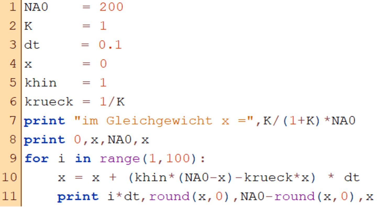
The system can be simulated using the TigerJython code. It is the numerical solution of a differential equation. However, not only whole apples but also fractions of apples are shifted between the two sides. Therefore, the rounded value for x is also output.

Commented code for TigerJython

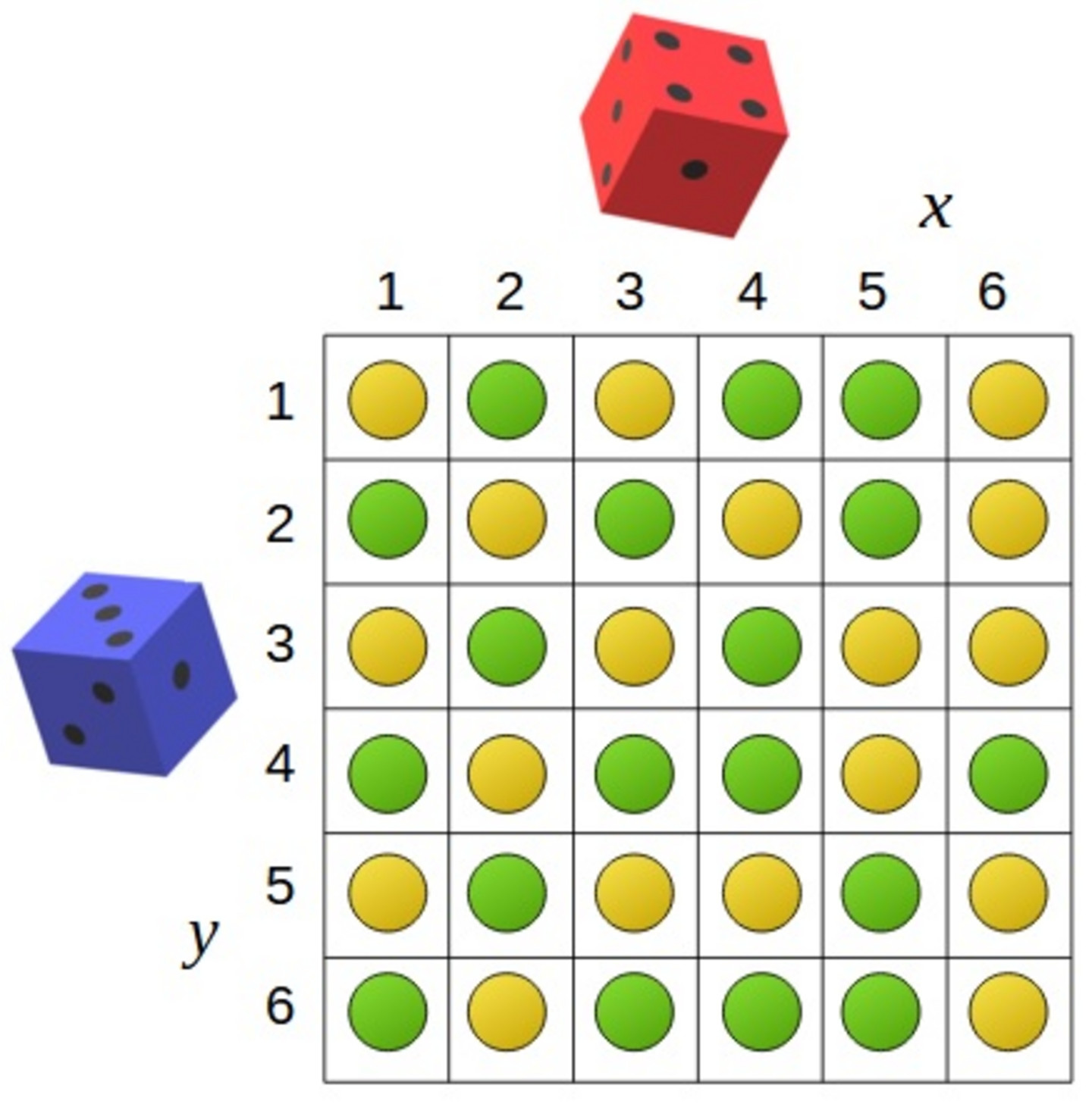
Alternatively, you can carry out a stochastic simulation. This involves determining a square on a 6x6 board with two dice and turning over a coin on this square, for example. Heads and tails represent reactant and product particles. This game can also be translated into a clear TigerJython code, as shown below.

Commented code for TigerJython

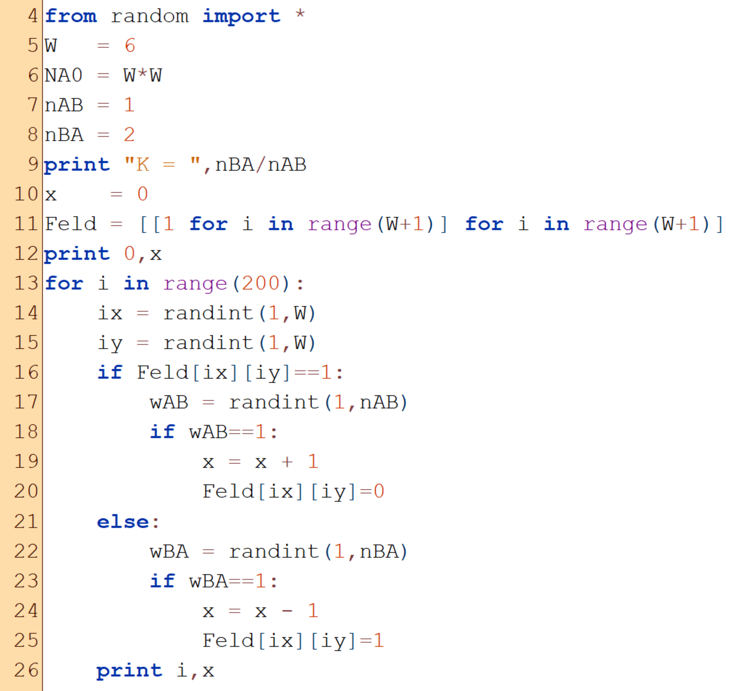
In this game or simulation, the reaction speed is the same in both directions, so that after some time there are the same number of edunkt and product particles on the board. If you continue to simulate, the number of particles fluctuates around the 50% value. The equilibrium constant is therefore always K=1. If you want to take other equilibrium constants into account, the probabilities for the outward and return reactions must differ, as implemented in the code below. The probability for the outward reaction is defined in lines 17/18 and for the backward reaction in lines 22/23.

Commented code for TigerJython